Linear Programming

It is an important optimization (maximization or minimization) technique used in decision making is business and everyday life for obtaining the maximum or minimum values as required of a linear expression to satisfying certain number of given linear restrictions.

Linear Programming Problem (LPP)

The linear programming problem in general calls for optimizing a linear function of variables called the objective function subject to a set of linear equations and/or linear inequations called the constraints or restrictions.

Objective Function

The function which is to be optimized (maximized/minimized) is called an objective function.

Constraints

The system of linear inequations (or equations) under which the objective function is to be optimized is called constraints.

Non-negative Restrictions

All the variables considered for making decisions assume non-negative values.

Mathematical Description of a General Linear Programming Problem

A general LPP can be stated as (Max/Min) z = c_lx_l + c₂x₂ + … + c_nx_n (Objective function) subject to constraints

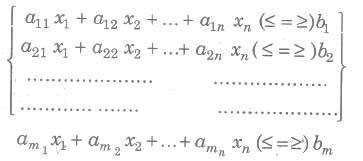
and the non-negative restrictions x_l, x₂,….., xn ≥ 0 where all a_l1, a_l2,…., amn; b_l, b₂,…., bm; c_l, c₂,…., cn are constants and x_l, x₂,…., xn are variables.

Slack and Surplus Variables

The positive variables which are added to left hand sides of the constraints to convert them into equalities are called the slack variables. The positive variables which are subtracted from the left hand sides of the constraints to convert them into equalities are called the surplus variables.

Important Definitions and Results

(i) Solution of a LPP A set of values of the variables x_l, x₂,…., x_n satisfying the constraints of a LPP is called a solution of the LPP.
(ii) Feasible Solution of a LPP A set of values of the variables x_l, x₂,…., x_n satisfying the constraints and non-negative restrictions of a LPP is called a feasible solution of the LPP.
(iii) Optimal Solution of a LPP A feasible solution of a LPP is said to, be optimal (or optimum), if it also optimizes the objective function of the problem.
(iv) Graphical Solution of a LPP The solution of a LPP obtained by graphical method i.e., by drawing the graphs corresponding to the constraints and the non-negative restrictions is called the graphical solution of a LPP.
(v) Unbounded Solution If the value of the objective function can be increased or decreased indefinitely, such solutions are called unbounded solutions.
(vi) Fundamental Extreme Point Theorem An optimum solution of a LPP, if it exists, occurs at one of the extreme points (i.e., corner points) of the convex Polygon of the set of all feasible solutions.

Solution of Simultaneous Linear Inequations

The graph or the solution set of a system of simultaneous linear inequations is the region containing the points (x, y) which satisfy all the inequations of the given system simultaneously.
To draw the graph of the simultaneous linear inequations, we find the region of the xy-plane, common to all the portions comprWng the solution sets of the given inequations. If there is no region common to all the solutions of the given inequations, we say that the solution set of the system of inequations is empty.

Note The solution set of simultaneous linear inequations may be an empty set or it may be the region bounded by the straight lines corresponding to given linear inequations or it may be an unbounded region with straight line boundaries.

Graphical Method to Solve a Linear Programming Problem

There are two techniques of solving a LPP by graphical method

1. Corner point method and

2. Iso-profit or Iso-cost method

1. Corner Point Method

This method of solving a LPP graphically is based on the principle of extreme point theorem.

Procedure to Solve a LPP Graphically by Corner Point Method

(i) Consider each constraint as an equation.
(ii) Plot each equation on graph, as each one will geometrically represent a straight line.
(iii) The common region, thus obtained satisfying all the constraints and the non-negative restrictions is called the feasible region. It is a convex polygon.
(iv) Determine the vertices (corner points) of the convex polygon. These vertices are known as the extreme points of corners of the feasible region.
(v) Find the values of the objective function at each of the extreme points. The point at which the value of the objective function is optimum (maximum or minimum) is the optimal solution of the given LPP.

2. Isom-profit or Iso-cost Method

Procedure to Solve a LPP Graphically by Iso-profit or Iso-cost Method

(i) Consider each constraint as an equation.
(ii) Plot each equation on graph as each one will geometrically represent a straight line.
(iii) The polygonal region so obtained, satisfying all the constraints and the non-negative restrictions is the convex set of all feasible solutions of the given LPP, which is also known as feasible region.
(iv) Determine the extreme points of the feasible region.
(v) Give some convenient value k to the objective function Z and draw the corresponding straight line in the xy-plane.
(vi) If the problem is of maximization, then draw lines parallel to the line Z = k and obtain a line which is farthest from the origin and has atleast one point common to the feasible region.
If the problem is of minimization, then draw lines parallel to the line Z = k and obtain a line, which is nearest to the origin and has atleast one point common to the feasible region.
(vii) The common point so obtained is the optimal solution of the given LPP.

Working Rule for Marking Feasible Region

Consider the constraint ax + by ≤ c, where c > 0.
First draw the straight line ax + by = c by joining any two points on it. For this find two convenient points satisfying this equation.This straight line divides the xy-plane in two parts. The inequation ax + by c will represent that part of the xy-plane which lies to that side of the line ax + by = c in which the origin lies.

Again, consider the constraint ax + by ≥ c, where c > 0.

Draw the straight line ax + by = c by joining any two points on it.

This straight line divides the xy-plane in two parts. The inequation ax + by ≥ c will represent that part of the xy-plane, which lies to that side of the line ax + by = c in which the origin does not lie.

Important Points to be Remembered

(i) Basic Feasible Solution

A BFS is a basic solution which also satisfies the non-negativity restrictions.

(ii) Optimum Basic Feasible Solution

A BFS is said to be optimum, if it also optimizes (Max or min) the objective function.

Important Definitions

1. Point Sets Point sets are sets whose elements are points or vectors in Eⁿ or Rⁿ (ndimensional euclidean space).

2. Hypersphere A hypersphere in En with centre at ‘a’ and radius ∈ > 0 is defined to be the set of points X = -{x:|x — a| = ∈}

3. An ∈ neighbourhood An & neighbourhood about the point ‘a is defined as the set of points lying inside the hypersphere with centre at ‘a’ and radius ∈ > 0.

4. An Interior Point A point ‘a’ is an interior point of the set S, if there exists an ∈ neighbourhood about ‘a’ which contains only points of the set S.

5. Boundary Point A point ‘a’ is a boundary point of the set S if every ∈ neighbourhood about ‘a’ contains points which are in the set and the points which are not in the set.

6. An Open. Set A set S is said to be an open set, if it contain only the interior points.

7. A Closed Set A set S is said to be a closed set, if it contains a its boundary points.

8. Lines In Eⁿ the line through the two points x₁ and x₂, x₁ ≠ x₂ is defined to be the set of points.
X = {x: x = λ x₁ + (1 — λ) x₂, for all real λ}

9. Line Segments In En, the line segment joining two point x₁ and x₂ is defined to be the set of points.

X = {x:x = λ x₁ + (1 — λ)x₂, 0 ≤ λ ≤ 1}

10. Hyperplane A hyperplane is defined as the set of points satisfying c₁x₁+ c₂x₂ + …+ cnxn = z (not all ci = 0) or cx = z for prescribed values of c₁, c₂,…, cn and z.

11. Open and Closed Half Spaces
A hyperplane divides the whole space En into three mutually disjoint sets given by
X₁ = {x : cx >z}
X₂ = {x : cx = z}
X₃ = {x : cx < z}
The sets x₁ and x₂ are called ‘open half spaces’. The sets {x : cx ≤ z} and { x : cx ≥ z} are called ‘closed half spaces’.

12. Parallel Hyperplanes Two hyperplanes c1x = z1 and c₂x = z₂ are said to be parallel, if they have the same unit normals i.e., if c₁ = Xc₂ for λ, λ being non-zero.

13. Convex Combination A convex combination of a finite number of points x₁, x₂,…., xn is defined as a point x = λ₁ x₁ + λ₂x₂ + …. + λnxn, where λi is real and ≥ 0, ∀ and

14. Convex Set A set of points is said to be convex, if for any two points in the set, the line segment joining these two points is also in the set.
or A set is convex, if the convex combination of any two points in the set, is also in the set.

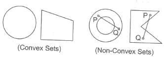
15 Extreme Point of a Convex Set A point x in a convex set c is called an ‘extreme point’, if x cannot be expressed as a convex combination of any two distinct points x₁ and x₂ in c.

16. Convex Hull The convex hull c(X) of any given set of points X is the set of all convex combinations of sets of points from X.

17. Convex Function A function f(x) is said to be strictly convex at x, if for any two other distinct points x₁ and x₂.

f{ λx₁ + (1 — λ)x₂} < λf(x₁) + (1— λ)f(x₂), where 0 < λ < 1.
And a function f(x) is strictly concave, if — f(x) is strictly convex.

18. Convex Polyhedron The set of all convex combinations of finite number of points is called the convex polyhedron generated by these points.

Important Points to be Remembered

(i) A hyperplane is a convex set.
(ii) The closed half spaces H₁ = {x : cx ≥ z} and H2 = {x : cx ≤ z} are convex sets.
(iii) The open half spaces : {x : cx > z} and {x : cx < z} are convex sets.
(iv) Intersection of two convex sets is also a convex sets.
(v) Intersection of any finite number of convex sets is also a convex set.
(vi) Arbitrary intersection of convex sets is also a convex set.
(vii) The set of all convex combinations of a finite number of points X₁, X₂,…., X_n is convex set.
(viii) A set C is convex, if and only if every convex linear combination of points in C, also belongs to C.
(ix) The set of all feasible solutions (if not empty) of a LPP is a convex set.
(x) Every basic feasible solution of the system Ax = b,x ≥ 0 is an extreme point of the convex set of feasible solutions and conversely.
(xi) If the convex set of the feasible solutions of Ax = b,x ≥ 0 is a convex polyhedron, then atleast one of the extreme points gives an optimal solution.
(xii) If the objective function of a LPP assumes its optimal value at more than one extreme point, then every convex combination of these extreme points gives the optimal value of the objective function.