A vector has direction and magnitude both but scalar has only magnitude.
The magnitude of a vector a is denoted by |a| or a. It is a non-negative scalar.

 

Equality of Vectors

Two vectors a and b are said to be equal written as a = b, if they have (i) same length (ii) the same or parallel support and (iii) the same sense.

Types of Vectors

(i) Zero or Null Vector

A vector whose initial and terminal points are coincident is called zero or null vector. It is denoted by 0.

(ii) Unit Vector

A vector whose magnitude is unity is called a unit vector which is denoted by nˆ

(iii) Free Vectors

If the initial point of a vector is not specified, then it is said to be a free vector.

(iv) Negative of a Vector

A vector having the same magnitude as that of a given vector a and the direction opposite to that of a is called the negative of a and it is denoted by —a.

(v) Like and Unlike Vectors

Vectors are said to be like when they have the same direction and unlike when they have opposite direction.

(vi) Collinear or Parallel Vectors

Vectors having the same or parallel supports are called collinear vectors.

(vii) Coinitial Vectors

Vectors having same initial point are called coinitial vectors.

(viii) Coterminous Vectors

Vectors having the same terminal point are called coterminous vectors.

(ix) Localized Vectors

A vector which is drawn parallel to a given vector through a specified point in space is called localized vector.

(x) Coplanar Vectors

A system of vectors is said to be coplanar, if their supports are parallel to the same plane. Otherwise they are called non-coplanar vectors.

(xi) Reciprocal of a Vector

A vector having the same direction as that of a given vector but magnitude equal to the reciprocal of the given vector is known as the reciprocal of a. i.e., if |a| = a, then |a^-1| = 1 / a.

 

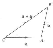
Addition of Vectors

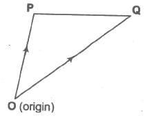
Let a and b be any two vectors. From the terminal point of a, vector b is drawn. Then, the vector from the initial point O of a to the terminal point B of b is called the sum of vectors a and b and is denoted by a + b. This is called the triangle law of addition of vectors.

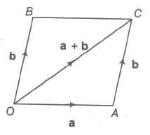
Parallelogram Law

Let a and b be any two vectors. From the initial point of a, vector b is drawn and parallelogram OACB is completed with OA and OB as adjacent sides. The vector OC is efined as the sum of a and b. This is called the parallelogram law of addition of vectors.

The sum of two vectors is also called their resultant and the process of addition as composition.

Properties of Vector Addition

(i) a + b = b + a (commutativity)
(ii) a + (b + c)= (a + b)+ c (associativity)
(iii) a+ O = a (additive identity)
(iv) a + (— a) = 0 (additive inverse)
(v) (k₁ + k₂) a = k₁ a + k₂a (multiplication by scalars)
(vi) k(a + b) = k a + k b (multiplication by scalars)
(vii) |a+ b| ≤ |a| + |b| and |a – b| ≥ |a| – |b|

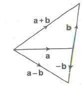
Difference (Subtraction) of Vectors

If a and b be any two vectors, then their difference a – b is defined as a + (- b).

Multiplication of a Vector by a Scalar

Let a be a given vector and λ be a scalar. Then, the product of the vector a by the scalar λ is λ a and is called the multiplication of vector by the scalar.

Important Properties

(i) |λ a| = |λ| |a|
(ii) λ O = O
(iii) m (-a) = – ma = – (m a)
(iv) (-m) (-a) = m a
(v) m (n a) = mn a = n(m a)
(vi) (m + n)a = m a+ n a
(vii) m (a+b) = m a + m b

Vector Equation of Joining by Two Points

Let P₁ (x₁, y₁, z₁) and P₂ (x₂, y₂, z₂) are any two points, then the vector joining P₁ and P₂ is the vector P₁ P₂.

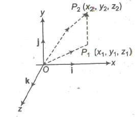
The component vectors of P and Q are

OP = x₁i + y₁j + z₁k and OQ = x₂i + y₂j + z₂k
i.e., P₁ P₂ = (x₂i + y₂j + z₂k) – (x₁i + y₁j + z₁k)
= (x₂ – x₁) i + (y₂ – y₁) j + (z₂ – z₁) k

Its magnitude is P₁ P₂ = √(x₂ – x₁)² + (y₂ – y₁)² + (z₂ – z₁)²

Position Vector of a Point

The position vector of a point P with respect to a fixed point, say O, is the vector OP. The fixed point is called the origin.
Let PQ be any vector. We have PQ = PO + OQ = — OP + OQ = OQ — OP = Position vector of Q — Position vector of P.

i.e., PQ = PV of Q — PV of P

Collinear Vectors

Vectors a and b are collinear, if a = λb, for some non-zero scalar λ.

 

Collinear Points

Let A, B, C be any three points.
Points A, B, C are collinear <=> AB, BC are collinear vectors.
<=> AB = λBC for some non-zero scalar λ.

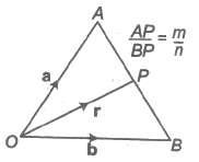
Section Formula

Let A and B be two points with position vectors a and b, respectively and OP= r.
(i) Let P be a point dividing AB internally in the ratio m : n. Then,
r = m b + n a / m + n

Also, (m + n) OP = m OB + n OA

(ii) The position vector of the mid-point of a and b is a + b / 2.
(iii) Let P be a point dividing AB externally in the ratio m : n. Then, r = m b + n a / m + n

Position Vector of Different Centre of a Triangle

(i) If a, b, c be PV’s of the vertices A, B, C of a ΔABC respectively, then the PV of the centroid G of the triangle is a + b + c / 3.
(ii) The PV of incentre of ΔABC is (BC)a + (CA)b + (AB)c / BC + CA + AB
(iii) The PV of orthocentre of ΔABC is a(tan A) + b(tan B) + c(tan C) / tan A + tan B + tan C

Scalar Product of Two Vectors

If a and b are two non-zero vectors, then the scalar or dot product of a and b is denoted by a * b and is defined as a * b = |a| |b| cos θ, where θ is the angle between the two vectors and 0 < θ < π .

(i) The angle between two vectors a and b is defined as the smaller angle θ between them, when they are drawn with the same initial point. Usually, we take 0 < θ < π.Angle between two like vectors is O and angle between two unlike vectors is π .
(ii) If either a or b is the null vector, then scalar product of the vector is zero.
(iii) If a and b are two unit vectors, then a * b = cos θ.
(iv) The scalar product is commutative i.e., a * b= b * a
(v) If i , j and k are mutually perpendicular unit vectors i , j and k, then i * i = j * j = k * k =1 and i * j = j * k = k * i = 0
(vi) The scalar product of vectors is distributive over vector addition.
(a) a * (b + c) = a * b + a * c (left distributive)
(b) (b + c) * a = b * a + c * a (right distributive)

Note Length of a vector as a scalar product If a be any vector, then the scalar product a * a = |a| |a| cosθ ⇒ |a|2 = a2 ⇒ a = |a| Condition of perpendicularity a * b = 0 <=> a ⊥ b, a and b being non-zero vectors.

Important Points to be Remembered

(i) (a + b) * (a – b) = |a|²2 – |b|²
(ii) |a + b|² = |a|²2 + |b|² + 2 (a * b)
(iii) |a – b|² = |a|²2 + |b|² – 2 (a * b)
(iv) |a + b|² + |a – b|² = (|a|²2 + |b|²) and |a + b|² – |a – b|² = 4 (a * b) or a * b = 1 / 4 [ |a + b|² – |a – b|² ]
(v) If |a + b| = |a| + |b|, then a is parallel to b.
(vi) If |a + b| = |a| – |b|, then a is parallel to b.
(vii) (a * b)² ≤ |a|²2 |b|²
(viii) If a = a₁i + a₂j + a₃k, then |a|² = a * a = a1² + a2 ² + a3 ² Or |a| = √a1 ² + a2 ² + a3 ²
(ix) Angle between Two Vectors
If θ is angle between two non-zero vectors, a, b, then we have a * b = |a| |b| cos θ cos θ = a * b / |a| |b| If a = a₁i + a₂j + a₃k and b = b₁i + b₂j + b₃k
Then, the angle θ between a and b is given by cos θ = a * b / |a| |b| = a₁b₁ + a₂b₂ + a₃b₃ / √a1 ² + a2 ² + a3 ² √b1 ² + b2 ² + b3 ²
(x) Projection and Component of a Vector
Projection of a on b = a * b / |a|
Projection of b on a = a * b / |a|
Vector component of a vector a on b

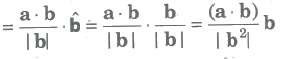
Similarly, the vector component of b on a = ((a * b) / |a²|) * a

(xi) Work done by a Force

The work done by a force is a scalar quantity equal to the product of the magnitude of the force and the resolved part of the displacement.

∴ F * S = dot products of force and displacement.

Suppose F₁, F₁,…, F_n are n forces acted on a particle, then during the displacement S of the particle, the separate forces do quantities of work F₁ * S, F₂ * S, F_n * S.

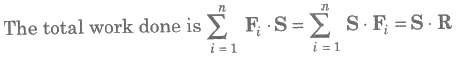
Here, system of forces were replaced by its resultant R.

 

Vector or Cross Product of Two Vectors

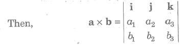
The vector product of the vectors a and b is denoted by a * b and it is defined as

a * b = (|a| |b| sin θ) n = ab sin θ n …..(i)

where, a = |a|, b= |b|, θ is the angle between the vectors a and b and n is a unit vector which is perpendicular to both a and b, such that a, b and n form a right-handed triad of vectors.

Important Points to be Remembered

(i) Let a = a₁i + a₂j + a₃k and b = b₁i + b₂j + b₃k

(ii) If a = b or if a is parallel to b, then sin θ = 0 and so a * b = 0.
(iii) The direction of a * b is regarded positive, if the rotation from a to b appears to be anticlockwise.
(iv) a * b is perpendicular to the plane, which contains both a and b. Thus, the unit vector perpendicular to both a and b or to the plane containing is given by n = a * b / |a * b| = a * b / ab sin θ
(v) Vector product of two parallel or collinear vectors is zero.
(vi) If a * b = 0, then a = O or b = 0 or a and b are parallel on collinear.
(vii) Vector Product of Two Perpendicular Vectors If θ = 900, then sin θ = 1, i.e. , a * b = (ab)n or |a * b| = |ab n| = ab
(viii) Vector Product of Two Unit Vectors
If a and b are unit vectors, then
a = |a| = 1, b = |b| = 1
∴ a * b = ab sin θ n = (sin theta;).n
(ix) Vector Product is not Commutative
The two vector products a * b and b * a are equal in magnitude but opposite in direction.
i.e., b * a =- a * b ……..(i)
(x) The vector product of a vector a with itself is null vector, i. e., a * a= 0.
(xi) Distributive Law For any three vectors a, b, c a * (b + c) = (a * b) + (a * c)
(xii) Area of a Triangle and Parallelogram
(a) The vector area of a ΔABC is equal to 1 / 2 |AB * AC| or 1 / 2 |BC * BA| or 1 / 2 |CB * CA|.
(b) The area of a ΔABC with vertices having PV’s a, b, c respectively, is 1 / 2 |a * b + b * c + c * a|.
(c) The points whose PV’s are a, b, c are collinear, if and only if a * b + b * c + c * a
(d) The area of a parallelogram with adjacent sides a and b is |a * b|.
(e) The area of a Parallelogram with diagonals a and b is 1 / 2 |a * b|.
(f) The area of a quadrilateral ABCD is equal to 1 / 2 |AC * BD|.
(xiii) Vector Moment of a Force about a Point

The vector moment of torque M of a force F about the point O is the vector whose magnitude is equal to the product of |F| and the perpendicular distance of the point O from the line of action of F.

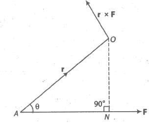
∴ M = r * F

where, r is the position vector of A referred to O.

(a) The moment of force F about O is independent of the choice of point A on the line of action of F.
(b) If several forces are acting through the same point A, then the vector sum of the moments of the separate forces about a point O is equal to the moment of their resultant force about O.
(xiv) The Moment of a Force about a Line

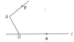
Let F be a force acting at a point A, O be any point on the given line L and a be the unit vector along the line, then moment of F about the line L is a scalar given by (OA x F) * a
(xv) Moment of a Couple
(a) Two equal and unlike parallel forces whose lines of action are different are said to constitute a couple.
(b) Let P and Q be any two points on the lines of action of the forces – F and F, respectively.

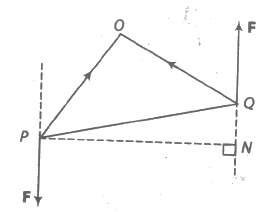
The moment of the couple = PQ x F

Scalar Triple Product

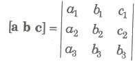
If a, b, c are three vectors, then (a * b) * c is called scalar triple product and is denoted by [a b c].
∴ [a b c] = (a * b) * c

 

Geometrical Interpretation of Scalar Triple Product

The scalar triple product (a * b) * c represents the volume of a parallelepiped whose coterminous edges are represented by a, b and c which form a right handed system of vectors.

Expression of the scalar triple product (a * b) * c in terms of components
a = a₁i + a₁j + a₁k, b = a₂i + a₂j + a₂k, c = a₃i + a₃j + a₃k is

Properties of Scalar Triple Products

1. The scalar triple product is independent of the positions of dot and cross i.e., (a * b) * c = a * (b * c).

2. The scalar triple product of three vectors is unaltered so long as the cyclic order of the vectors remains unchanged.
i.e., (a * b) * c = (b * c) * a= (c * a) * b or [a b c] = [b c a] = [c a b]

.3. The scalar triple product changes in sign but not in magnitude, when the cyclic order is changed.
i.e., [a b c] = – [a c b] etc.

4. The scalar triple product vanishes, if any two of its vectors are equal.
i.e., [a a b] = 0, [a b a] = 0 and [b a a] = 0.

5. The scalar triple product vanishes, if any two of its vectors are parallel or collinear.

6. For any scalar x, [x a b c] = x [a b c]. Also, [x a yb zc] = xyz [a b c].

7. For any vectors a, b, c, d, [a + b c d] = [a c d] + [b c d]

8. [i j k] = 1

11. Three non-zero vectors a, b and c are coplanar, if and only if [a b c] = 0.

12. Four points A, B, C, D with position vectors a, b, c, d respectively are coplanar, if and only if [AB AC AD] = 0.
i.e., if and only if [b — a c— a d— a] = 0.

13. Volume of parallelepiped with three coterminous edges a, b,c is | [a b c] |.

14. Volume of prism on a triangular base with three coterminous edges a,b,c is 1/2 | [a b c] |.

15. Volume of a tetrahedron with three coterminous edges a, b,c is 1 / 6 | [a b c] |.

16. If a, b, c and d are position vectors of vertices of a tetrahedron, then Volume = 1 / 6 [b — a c — a d — a].

Vector Triple Product

If a, b, c be any three vectors, then (a * b) * c and a * (b * c) are known as vector triple product.
∴ a * (b * c)= (a * c)b — (a * b) c and (a * b) * c = (a * c)b — (b * c) a

Important Properties

(i) The vector r = a * (b * c) is perpendicular to a and lies in the plane b and c.

(ii) a * (b * c) ≠ (a * b) * c, the cross product of vectors is not associative.

(iii) a * (b * c)= (a * b) * c, if and only if and only if (a * c)b — (a * b) c = (a * c)b — (b * c) a, if and only if c = (b * c) / (a * b) * a Or if and only if vectors a and c are collinear.

Reciprocal System of Ve ctors

Let a, b and c be three non-coplanar vectors and let a’ = b * c / [a b c], b’ = c * a / [a b c], c’ = a * b / [a b c]
Then, a’, b’ and c’ are said to form a reciprocal system of a, b and c.

Properties of Reciprocal System

(i) a * a’ = b * b’= c * c’ = 1
(ii) a * b’= a * c’ = 0, b * a’ = b * c’ = 0, c * a’ = c * b’= 0
(iii) [a’, b’, c’] [a b c] = 1 ⇒ [a’ b’ c’] = 1 / [a b c]
(iv) a = b’ * c’ / [a’, b’, c’], b = c’ * a’ / [a’, b’, c’], c = a’ * b’ / [a’, b’, c’]
Thus, a, b, c is reciprocal to the system a’, b’ ,c’.
(v) The orthonormal vector triad i, j, k form self reciprocal system.
(vi) If a, b, c be a system of non-coplanar vectors and a’, b’, c’ be the reciprocal system of vectors, then any vector r can be expressed as r = (r * a’ )a + (r * b’)b + (r * c’)c.

Linear Combination of Vectors

Let a, b, c,… be vectors and x, y, z, … be scalars, then the expression x a yb + z c + … is called a linear combination of vectors a, b, c,….

Collinearity of Three Points

The necessary and sufficient condition that three points with PV’s b, c are collinear is that there exist three scalars x, y, z not all zero such that xa + yb + zc ⇒ x + y + z = 0.

Coplanarity of Four Points

The necessary and sufficient condition that four points with PV’s a, b, c, d are coplanar, if there exist scalar x, y, z, t not all zero, such that xa + yb + zc + td = 0 rArr; x + y + z + t = 0.
If r = xa + yb + zc…

Then, the vector r is said to be a linear combination of vectors a, b, c,….

Linearly Independent and Dependent System of Vectors

(i) The system of vectors a, b, c,… is said to be linearly dependent, if there exists a scalars x, y, z, … not all zero, such that xa + yb + zc + … = 0.
(ii) The system of vectors a, b, c, … is said to be linearly independent, if xa + yb + zc + td = 0 rArr; x + y + z + t… = 0.

Important Points to be Remembered

(i) Two non-collinear vectors a and b are linearly independent.
(ii) Three non-coplanar vectors a, b and c are linearly independent.
(iii) More than three vectors are always linearly dependent.

 

Resolution of Components of a Vector in a Plane

Let a and b be any two non-collinear vectors, then any vector r coplanar with a and b, can be uniquely expressed as r = x a + y b, where x, y are scalars and x a, y b are called components of vectors in the directions of a and b, respectively.

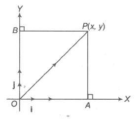
∴ Position vector of P(x, y) = x i + y j.
OP² = OA² + AP² = |x|² + |y|² = x² + y²
OP = √x² + y². This is the magnitude of OP.

where, x i and y j are also called resolved parts of OP in the directions of i and j, respectively.

Vector Equation of Line and Plane

(i) Vector equation of the straight line passing through origin and parallel to b is given by r = t b, where t is scalar.
(ii) Vector equation of the straight line passing through a and parallel to b is given by r = a + t b, where t is scalar.
(iii) Vector equation of the straight line passing through a and b is given by r = a + t(b – a), where t is scalar.
(iv) Vector equation of the plane through origin and parallel to b and c is given by r = s b + t c, where s and t are scalars.
(v) Vector equation of the plane passing through a and parallel to b and c is given by r = a + sb + t c, where s and t are scalars.
(vi) Vector equation of the plane passing through a, b and c is r = (1 – s – t)a + sb + tc, where s and t are scalars.

Bisectors of the Angle between Two Lines

(i) The bisectors of the angle between the lines r = λa and r = μb are given by r = &lamba; (a / |a| &plumsn; b / |b|)
(ii) The bisectors of the angle between the lines r = a + λb and r = a + μc are given by r = a + &lamba; (b / |b| &plumsn; c / |c|)