-
1.Relations and Functions
- Revision – Functions and its Types
- Revision – Functions Types
- Revision – Sum Related to Relations
- Revision – Sums Related to Relations, Domain and Range
- Cartesian Product of Sets, Relation, Domain, Range, Inverse of Relation, Types of Relations
- Functions, Intervals
- Domain
- Problem Based on finding Domain and Range
- Types of Real function
- Odd & Even Function, Composition of Function
- Chapter Notes – Relations and Functions
-
2.Inverse Trigonometric Functions
- Revision – Introduction, Some Identities and Some Sums
- Revision – Some Sums Related to Trigonometry Identities, trigonometry Functions Table and Its Quadrants
- Revision – Trigonometrical Identities-Some important relations and Its related Sums
- Revision – Sums Related to Trigonometrical Identities
- Revision – Some Trigonometric Identities and its related Sums
- Revision – Trigonometry Equations
- Revision – Sum Based on Trigonometry Equations
- Introduction to Inverse Trigonometry Function, Range, Domain, Question based on Principal Value
- Property -1 of Inverse trigo function
- Property -2 to 4 of Inverse trigo function
- Questions based on properties of Inverse trigo function
- Question based on useful substitution
- Numerical problems
- Numerical problems
- Numerical problems , introduction to Differentiation
- Chapter Notes – Inverse Trigonometric Functions
-
3.Matrices
-
4.Determinants
-
5.Continuity
-
6.Differentiation
- Introduction to Differentiation
- Important formula’s
- Numerical problems
- Numerical problems
- Differentiation by using trigonometric substitution
- Differentiation of implicit function
- Differentiation of logarthmetic function
- Differentiation of log function
- Infinite series & parametric function
- Infinite series & parametric function
- Higher order derivatives
- Differentiation of function of a function
- Numerical problems
- Numerical problems
-
7.Mean Value Theorem
-
8.Applications of Derivatives
-
9.Increasing and Decreasing Function
-
10.Tangents and Normal
-
11.Maxima and Minima
-
12.Integrations
- Introduction to Indefinite Integration
- Integration by substitution
- Numerical problems on Substitution
- Numerical problems on Substitution
- Integration various types of particular function (Identities)
- Integration by parts-1
- Integration by parts-2
- Integration by parts-2
- Integration by parts-2
- ILATE Rule
- Integration of some special function
- Integration of some special function
- Integration by substitution using trigonometric
- Evaluation of some specific Integration
- Evaluation of some specific Integration
- Integration by partial fraction
- Integration of some special function
- Numerical Problems based on partial fraction
- Chapter Notes – Integrals
-
13.Definite Integrals
- Introduction
- Properties of Definite Integration
- Numerical problem based on properties
- Area under the curve
- Area under the curve (Ellipse)
- Area under the curve (Parabola)
- Area under the curve (Parabola & Circle)
- Area bounded by lines
- Numerical problems
- Area under the curve (Circle )
- Chapter Notes – Application of Integrals
-
14.Differential Equations
-
15.Vectors
- Introduction , Basic concepts , types of vector
- Position vector, distance between two points, section formula
- Numerical problem
- collinearity of points and coplanarity of vector
- Direction cosine
- Projection , Dot product, Cauchy- Schwarz inequality
- Numerical problem (dot product)
- Vector (Cross) product , Lagrange’s Identity
- Numerical problem (cross product)
- Numerical problem (cross product)
- Numerical problem (cross product)
- Chapter Notes – Vectors
-
16.Three Dimensional Geometry
- Introduction to 3D, axis in 3D, plane in 3D, Distance between two points
- Numerical problems , section formula , centroid of a triangle
- projection , angle between two lines
- Numerical Problem based on Direction ratio & cosine
- locus of any point
- Numerical Problem based on locus
- Chapter Notes – Three Dimensional Geometry
-
17.Direction Cosine
-
18.Plane
-
19.Straight Lines
- Revision – Introduction, Equation of Line, Slope or Gradient of a line
- Revision – Sums Related to Finding the Slope, Angle Between two Lines
- Revision – Cases for Angle B/w two Lines, Different forms of Line Equation
- Revision – Sums Related Finding the Equation of Line
- Revision – Sums based on Previous Concepts of Straight line
- Revision – Parametric Form of a Straight Line
- Revision – Sums Related to Parametric Form of a Straight Line
- Revision – Sums Based on Concurrent of lines, Angle b/w Two Lines
- Revision – Different condition for Angle b/w two lines
- Revision – Sums Based on Angle b/w Two Lines
- Revision – Equation of Straight line Passes Through a Point and Make an Angle with Another Line
- Revision – Sums Based on Equation of Straight line Passes Through a Point and Make an Angle with Another Line
- Revision – Sums Based on Equation of Straight line Passes Through a Point and Make an Angle with Another Line
- Revision – Finding the Distance of a point from the line
- Revision – Sum Based on Finding the Distance of a point from the line and B/w Two Parallel Lines
- Introduction to straight line , symmetric form , Angle between the lines
- Numerical Problem
- Angle between two lines
- Unsymmetric form of Line
- Numerical problem , perpendicular distance of a point from a line
- Numerical Problem
- Numerical problem , Condition for a line lie on a plane
-
20.Straight Lines (Vector)
-
21.Linear Programming
-
22.Probability
- Introduction to probability
- Types of events
- Numerical problems
- Conditional probability
- Numerical problems
- Numerical problems (conditional Probability)
- Numerical problems (conditional Probability)
- Numerical problems (conditional Probability)
- Numerical problems (conditional Probability)
- Bayes’ Theorem
- Numerical problem ( conditional Probability)
- Numerical problem ( Baye’s Theorem)
- Numerical problem ( Baye’s Theorem)
- Numerical problem ( Baye’s Theorem)
- Mean and Variance of a random variable
- Mean and Variance of a random variable
- Mean and Variance of a random variable
- Mean and Variance of a discrete random variable
- Numerical problem
- Bernoulli’s Trials & Binomial Distribution
- Numerical problem
- Mean and Variance of Binomial Distribution
- Chapter Notes – Probability
-
23.Limits
-
24.Partial Fractions
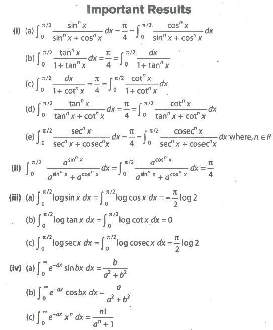
Chapter Notes – Application of Integrals
Let f(x) be a function defined on the interval [a, b] and F(x) be its anti-derivative. Then,
![]()
The above is called the second fundamental theorem of calculus.
![]() is defined as the definite integral of f(x) from x = a to x = b. The numbers and b are called limits of integration. We write
is defined as the definite integral of f(x) from x = a to x = b. The numbers and b are called limits of integration. We write
![]()
Evaluation of Definite Integrals by Substitution
Consider a definite integral of the following form
![]()
Step 1 Substitute g(x) = t
⇒ g ‘(x) dx = dt
Step 2 Find the limits of integration in new system of variable i.e.. the lower limit is g(a) and the upper limit is g(b) and the g(b) integral is now![]()
Step 3 Evaluate the integral, so obtained by usual method.
Properties of Definite Integral
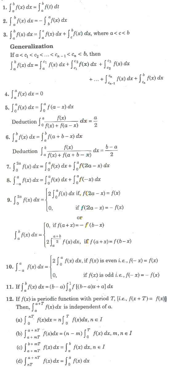
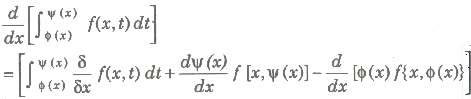
13. Leibnitz Rule for Differentiation Under Integral Sign
(a) If Φ(x) and ψ(x) are defined on [a, b] and differentiable for every x and f(t) is continuous, then
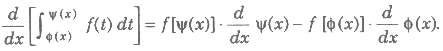
(b) If Φ(x) and ψ(x) are defined on [a, b] and differentiable for every x and f(t) is continuous, then
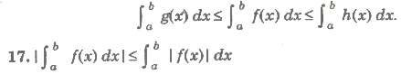
14. If f(x) ≥ 0 on the interval [a, b], then![]()
15. If (x) ≤ Φ(x) for x ∈ [a, b], then ![]()
16. If at every point x of an interval [a, b] the inequalities g(x) ≤ f(x) ≤ h(x) are fulfilled, then
18. If m is the least value and M is the greatest value of the function f(x) on the interval [a, bl. (estimation of an integral), then
![]()
19. If f is continuous on [a, b], then there exists a number c in [a, b] at which
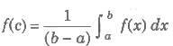
is called the mean value of the function f(x) on the interval [a, b].
20. If f22 (x) and g2 (x) are integrable on [a, b], then
![]()
21. Let a function f(x, α) be continuous for a ≤ x ≤ b and c ≤ α ≤ d.
Then, for any α ∈ [c, d], if
![]()
22. If f(t) is an odd function, then![]() is an even function.
is an even function.
23. If f(t) is an even function, then![]() is an odd function.
is an odd function.
24. If f(t) is an even function, then for non-zero a,![]() is not necessarily an odd function. It will be an odd function, if
is not necessarily an odd function. It will be an odd function, if
![]()
25. If f(x) is continuous on [a, α], then![]() is called an improper integral and is defined as
is called an improper integral and is defined as![]()
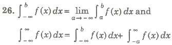
27. Geometrically, for f(x) > 0, the improper integral![]() gives area of the figure bounded by the curve y = f(x), the axis and the straight line x = a.
gives area of the figure bounded by the curve y = f(x), the axis and the straight line x = a.
Integral Function
Let f(x) be a continuous function defined on [a, b], then a function φ(x) defined by![]() is called the integral function of the function f.
is called the integral function of the function f.
Properties of Integral Function
1. The integral function of an integrable function is continuous.
2. If φ(x) is the integral function of continuous function, then φ(x) is derivable and of φ ‘ = f(x) for all x ∈ [a, b].
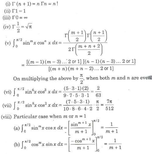
Gamma Function
If n is a positive rational number, then the improper integral![]() is defined as a gamma function and it is denoted by Γn
is defined as a gamma function and it is denoted by Γn
![]()
Properties of Gamma Function
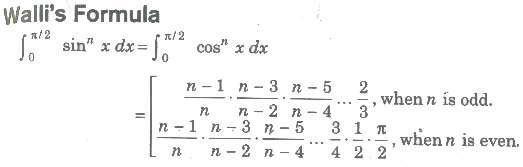
Summation of Series by Definite Integral
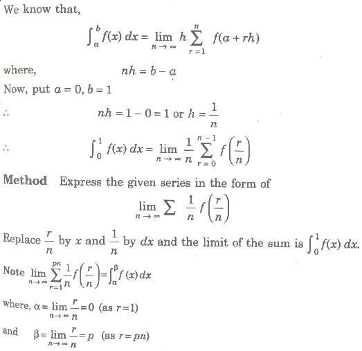
The method to evaluate the integral, as limit of the sum of an infinite series is known as integration by first principle.
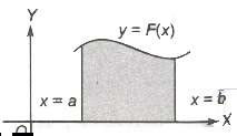
Area of Bounded Region
The space occupied by the curve along with the axis, under the given condition is called area of bounded region.
(i) The area bounded by the curve y = F(x) above the X-axis and between the lines x = a, x = b is given by ![]()
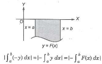
(ii) If the curve between the lines x = a, x = b lies below the X-axis, then the required area is given by
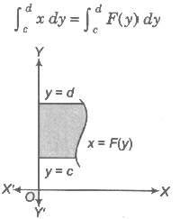
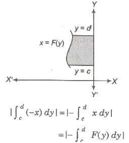
(iii) The area bounded by the curve x = F(y) right to the Y-axis and the lines y = c, y = d is given by
(iv) If the curve between the lines y = c, y = d left to the Y-axis, then the area is given by
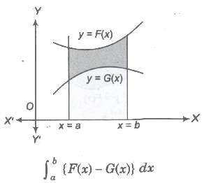
(v) Area bounded by two curves y = F (x) and y = G (x) between x = a and x = b is given by
(vi) Area bounded by two curves x = f(y) and x = g(y) between y=c and y=d is given by![]()
(vii) If F (x) ≥. G (x) in [a, c] and F (x) ≤ G (x) in [c,d], where a < c < b, then area of the region bounded by the curves is given as
![]()
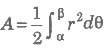
Area of Curves Given by Polar Equations
Let f(θ) be a continuous function, θ ∈ (a, α), then the are t bounded by the curve r = f(θ) and <β) is
Area of Parametric Curves
Let x = φ(t) and y = ψ(t) be two parametric curves, then area bounded by the curve, X-axis and ordinates x = φ(t1), x = ψ(t2) is
![]()
Volume and Surface Area
If We revolve any plane curve along any line, then solid so generated is called solid of revolution.
1. Volume of Solid Revolution
1. The volume of the solid generated by revolution of the area bounded by the curve y = f(x), the axis of x and the ordinates![]() it being given that f(x) is a continuous a function in the interval (a, b).
it being given that f(x) is a continuous a function in the interval (a, b).
2. The volume of the solid generated by revolution of the area bounded by the curve x = g(y), the axis of y and two abscissas y = c and y = d is![]() it being given that g(y) is a continuous function in the interval (c, d).
it being given that g(y) is a continuous function in the interval (c, d).
Surface of Solid Revolution
(i) The surface of the solid generated by revolution of the area bounded by the curve y = f(x), the axis of x and the ordinates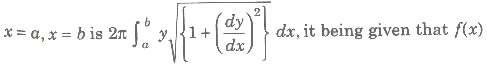 is a continuous function in the interval (a, b).
(ii) The surface of the solid generated by revolution of the area bounded by the curve x = f (y), the axis of y and y = c, y = d is![]() continuous function in the interval (c, d).
continuous function in the interval (c, d).
Curve Sketching
1. symmetry
1. If powers of y in a equation of curve are all even, then curve is symmetrical about Xaxis.
2. If powers of x in a equation of curve are all even, then curve is symmetrical about Yaxis.
3. When x is replaced by -x and y is replaced by -y, then curve is symmetrical in opposite quadrant.
4. If x and y are interchanged and equation of curve remains unchanged curve is symmetrical about line y = x.
2. Nature of Origin
1. If point (0, 0) satisfies the equation, then curve passes through origin.
2. If curve passes through origin, then equate low st degree term to zero and get equation of tangent. If there are two tangents, then origin is a double point.
3. Point of Intersection with Axes
1. Put y = 0 and get intersection with X-axis, put x = 0 and get intersection with Y-axis.
2. Now, find equation of tangent at this point i. e. , shift origin to the point of intersection and equate the lowest degree term to zero.
3. Find regions where curve does not exists. i. e., curve will not exit for those values of variable when makes the other imaginary or not defined.
4. Asymptotes
1. Equate coefficient of highest power of x and get asymptote parallel to X-axis.
2. Similarly equate coefficient of highest power of y and get asymptote parallel to Y-axis.
5. The Sign of (dy/dx)
Find points at which (dy/dx) vanishes or becomes infinite. It gives us the points where tngent is parallel or perpendicular to the X-axis.
6. Points of Inflexion
![]() and solve the resulting equation.If some point of inflexion is there, then locate it exactly.
and solve the resulting equation.If some point of inflexion is there, then locate it exactly.
Taking in consideration of all above information, we draw an approximate shape of the curve
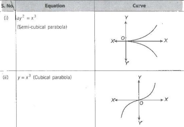
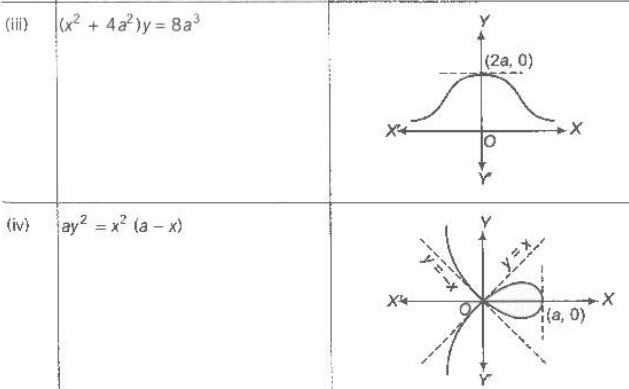
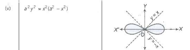
Shape of Some Curves is Given Below