A matrix is a rectangular arrangement of numbers (real or complex) which may be represented as

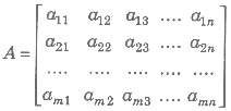
matrix is enclosed by [ ] or ( ) or | | | | Compact form the above matrix is represented by [a_ij]_{m x n} or A = [a_ij].
1. Element of a Matrix The numbers a₁₁, a₁₂ … etc., in the above matrix are known as the element of the matrix, generally represented as a_ij , which denotes element in ith row and jth column.
2. Order of a Matrix In above matrix has m rows and n columns, then A is of order m x n.

Types of Matrices

1. Row Matrix A matrix having only one row and any number of columns is called a row matrix.
2. Column Matrix A matrix having only one column and any number of rows is called column matrix.
3. Rectangular Matrix A matrix of order m x n, such that m ≠ n, is called rectangular matrix.
4. Horizontal Matrix A matrix in which the number of rows is less than the number of columns, is called a horizontal matrix.
5. Vertical Matrix A matrix in which the number of rows is greater than the number of columns, is called a vertical matrix.
6. Null/Zero Matrix A matrix of any order, having all its elements are zero, is called a null/zero matrix. i.e., a_ij = 0, ∀ i, j
7. Square Matrix A matrix of order m x n, such that m = n, is called square matrix.
8. Diagonal Matrix A square matrix A = [a_ij]_{m x n}, is called a diagonal matrix, if all the elements except those in the leading diagonals are zero, i.e., a_ij = 0 for i ≠ j. It can be
represented as A = diag[a₁₁ a₂₂… a_nn]
9. Scalar Matrix A square matrix in which every non-diagonal element is zero and all diagonal elements are equal, is called scalar matrix.
i.e., in scalar matrix a_ij = 0, for i ≠ j and a_ij = k, for i = j
10. Unit/Identity Matrix A square matrix, in which every non-diagonal element is zero and every diagonal element is 1, is called, unit matrix or an identity matrix.

11. Upper Triangular Matrix A square matrix A = a[_ij]_{n x n} is called a upper triangular matrix, if a[_ij], = 0, ∀ i > j.
12. Lower Triangular Matrix A square matrix A = a[_ij]_{n x n} is called a lower triangular matrix, if a[_ij], = 0, ∀ i < j.
13. Submatrix A matrix which is obtained from a given matrix by deleting any number of rows or columns or both is called a submatrix of the given matrix.
14. Equal Matrices Two matrices A and B are said to be equal, if both having same order and corresponding elements of the matrices are equal.
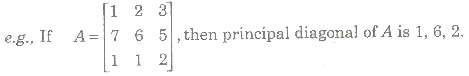
15. Principal Diagonal of a Matrix In a square matrix, the diagonal from the first element of
the first row to the last element of the last row is called the principal diagonal of a matrix.

16. Singular Matrix A square matrix A is said to be singular matrix, if determinant of A denoted by det (A) or |A| is zero, i.e., |A|= 0, otherwise it is a non-singular matrix.

Algebra of Matrices

1. Addition of Matrices

Let A and B be two matrices each of order m x n. Then, the sum of matrices A + B is defined only if matrices A and B are of same order.
If A = [a_ij]_{m x n} , A = [a_ij]_{m x n}
Then, A + B = [a_ij + b_ij]_{m x n}

Properties of Addition of Matrices

If A, B and C are three matrices of order m x n, then

1. Commutative Law A + B = B + A
2. Associative Law (A + B) + C = A + (B + C)
3. Existence of Additive Identity A zero matrix (0) of order m x n (same as of A), is additive identity, if A + 0 = A = 0 + A
4. Existence of Additive Inverse If A is a square matrix, then the matrix (- A) is called additive inverse, if A + ( – A) = 0 = (- A) + A
5. Cancellation Law
A + B = A + C ⇒ B = C (left cancellation law)
B + A = C + A ⇒ B = C (right cancellation law)

2. Subtraction of Matrices

Let A and B be two matrices of the same order, then subtraction of matrices, A – B, is defined as A – B = [a_ij – b_ij]_{n x n}, where A = [a_ij]_{m x n}, B = [b_ij]_{m x n}

3. Multiplication of a Matrix by a Scalar

Let A = [a_ij]_{m x n} be a matrix and k be any scalar. Then, the matrix obtained by multiplying each element of A by k is called the scalar multiple of A by k and is denoted by kA, given as kA= [ka_ij]_{m x n}

Properties of Scalar Multiplication If A and B are matrices of order m x n, then

1. k(A + B) = kA + kB
2. (k₁ + k₂)A = k₁A + k₂A
3. k₁k₂A = k₁(k₂A) = k₂(k₁A)
4. (- k)A = – (kA) = k( – A)

4. Multiplication of Matrices

Let A = [a_ij]_{m x n} and B = [b_ij]n x p are two matrices such that the number of columns of A is equal to the number of rows of B, then multiplication of A and B is denoted by AB, is given by

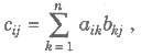
where c_ij is the element of matrix C and C = AB

Properties of Multiplication of Matrices

1. Commutative Law Generally AB ≠ BA
2. Associative Law (AB)C = A(BC)
3. Existence of multiplicative Identity A.I = A = I.A, I is called multiplicative Identity.
4. Distributive Law A(B + C) = AB + AC
5. Cancellation Law If A is non-singular matrix, then
AB = AC ⇒ B = C (left cancellation law)
BA = CA ⇒B = C (right cancellation law)
6. AB = 0, does not necessarily imply that A = 0 or B = 0 or both A and B = 0

 

Important Points to be Remembered

(i) If A and B are square matrices of the same order, say n, then both the product AB and BA are defined and each is a square matrix of order n.
(_ii) In the matrix product AB, the matrix A is called premultiplier (prefactor) and B is called postmultiplier (postfactor).
(_iii) The rule of multiplication of matrices is row column wise (or → ↓ wise) the first row of AB is obtained by multiplying the first row of A with first, second, third,… columns of B respectively; similarly second row of A with first, second, third, … columns of B, respectively and so on.

Positive Integral Powers of a Square Matrix

Let A be a square matrix. Then, we can define

1. A_{^{n + 1}} = A_ⁿ. A, where n ∈ N.
2. A^m. A_ⁿ = A^{m + n}
3. (Am)_ⁿ = A^mn, ∀ m, n ∈ N

Matrix Polynomial

Let f(x)= a^₀xⁿ + a1x^{n – 1 -1} + a2x^{n – 2} + … + an. Then f(A)= a₀Aⁿ + a₁A^{n – 2} + … + a_nI_n is called the matrix polynomial.

Transpose of a Matrix

Let A = [a_ij]_{m x n}, be a matrix of order m x n. Then, the n x m matrix obtained by interchanging the rows and columns of A is called the transpose of A and is denoted by ’or A^T.
A’ = AT = [a_ij]_{n x m}

Properties of Transpose

1. (A’)’ = A
2. (A + B)’ = A’ + B’
3. (AB)’ = B’A’
4. (KA)’ = kA’
5. (A^N)’ = (A’)^N
6. (ABC)’ = C’ B’ A’

Symmetric and Skew-Symmetric Matrices

1. A square matrix A = [a_ij]<<, is said to be symmetric, if A’ = A.
i.e., a_ij = a_ji , ∀i and j.
2. A square matrix A is said to be skew-symmetric matrices, if i.e., a_ij = — a_ji, di and j

Properties of Symmetric and Skew-Symmetric Matrices

1. Elements of principal diagonals of a skew-symmetric matrix are all zero. i.e., a_ii = — a_ii 2< = 0 or a_ii = 0, for all values of i.
2. If A is a square matrix, then
(a) A + A’ is symmetric.
(b) A — A’ is skew-symmetric matrix.

3. If A and B are two symmetric (or skew-symmetric) matrices of same order, then A + B is also symmetric (or skew-symmetric).
4. If A is symmetric (or skew-symmetric), then kA (k is a scalar) is also symmetric for skew-symmetric matrix.
5. If A and B are symmetric matrices of the same order, then the product AB is symmetric, iff BA = AB.
6. Every square matrix can be expressed uniquely as the sum of a symmetric and a skewsymmetric matrix.
7. The matrix B’ AB is symmetric or skew-symmetric according as A is symmetric or skew-symmetric matrix.
8. All positive integral powers of a symmetric matrix are symmetric.
9. All positive odd integral powers of a skew-symmetric matrix are skew-symmetric and positive even integral powers of a skew-symmetric are symmetric matrix.
10. If A and B are symmetric matrices of the same order, then
(a) AB – BA is a skew-symmetric and
(b) AB + BA is symmetric.

 

11. For a square matrix A, AA’ and A’ A are symmetric matrix.

Trace of a Matrix

The sum of the diagonal elements of a square matrix A is called the trace of A, denoted by trace (A) or tr (A).

Properties of Trace of a Matrix

1. Trace (A ± B)= Trace (A) ± Trace (B)
2. Trace (kA)= k Trace (A)
3. Trace (A’ ) = Trace (A)
4. Trace (I_n)= n
5. Trace (0) = 0
6. Trace (AB) ≠ Trace (A) x Trace (B)
7. Trace (AA’) ≥ 0

Conjugate of a Matrix

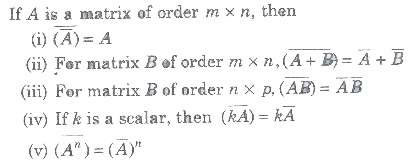
If A is a matrix of order m x n, then

Transpose Conjugate of a Matrix

The transpose of the conjugate of a matrix A is called transpose conjugate of A and is denoted by A⁰ or A^{*.
i.e., (A’) = A‘ = A0 or A*}

Properties of Transpose Conjugate of a Matrix

(i) (A^{*)* = A
(ii) (A + B)* = A* + B*
(iii) (kA)* = kA*
(iv) (AB)* = B*A*
(V) (An)* = (A*)n}

Some Special Types of Matrices

1. Orthogonal Matrix

A square matrix of order n is said to be orthogonal, if AA’ = I_n = A’A Properties of Orthogonal Matrix
(i) If A is orthogonal matrix, then A’ is also orthogonal matrix.
(ii) For any two orthogonal matrices A and B, AB and BA is also an orthogonal matrix.
(iii) If A is an orthogonal matrix, A^-1 is also orthogonal matrix.

2. ldempotent Matrix

A square matrix A is said to be idempotent, if A² = A.

Properties of Idempotent Matrix

(i) If A and B are two idempotent matrices, then
• AB is idempotent, if AB = BA.
• A + B is an idempotent matrix, iff AB = BA = 0
• AB = A and BA = B, then A² = A, B² = B
(ii)
• If A is an idempotent matrix and A + B = I, then B is an idempotent and AB = BA= 0.
• Diagonal (1, 1, 1, …,1) is an idempotent matrix.
• If I₁, I₂ and I₃ are direction cosines, then

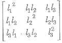
is an idempotent as |Δ|² = 1.
A square matrix A is said to be involutory, if A² = I

4. Nilpotent Matrix

A square matrix A is said to be nilpotent matrix, if there exists a positive integer m such that A² = 0. If m is the least positive integer such that A^m = 0, then m is called the index of the nilpotent matrix A.

5. Unitary Matrix

A square matrix A is said to be unitary, if A‘A = I

Hermitian Matrix

A square matrix A is said to be hermitian matrix, if A = A^* or = a_ij, for a_ji only.

Properties of Hermitian Matrix

1. If A is hermitian matrix, then kA is also hermitian matrix for any non-zero real number k.
2. If A and B are hermitian matrices of same order, then λ_λA + λB, also hermitian for any non-zero real number λ_λ, and λ.
3. If A is any square matrix, then AA^* and A^* A are also hermitian.
4. If A and B are hermitian, then AB is also hermitian, iff AB = BA
5. If A is a hermitian matrix, then A is also hermitian.
6. If A and B are hermitian matrix of same order, then AB + BA is also hermitian.
7. If A is a square matrix, then A + A^* is also hermitian,
8. Any square matrix can be uniquely expressed as A + iB, where A and B are hermitian matrices.

Skew-Hermitian Matrix

A square matrix A is said to be skew-hermitian if A^* = – A or a_ji for every i and j.

Properties of Skew-Hermitian Matrix

1. If A is skew-hermitian matrix, then kA is skew-hermitian matrix, where k is any nonzero real number.
2. If A and B are skew-hermitian matrix of same order, then λ_λA + λ₂B is also skewhermitian for any real number λ_λ and λ₂.
3. If A and B are hermitian matrices of same order, then AB — BA is skew-hermitian.
4. If A is any square matrix, then A — A^* is a skew-hermitian matrix.
5. Every square matrix can be uniquely expressed as the sum of a hermitian and a skewhermitian matrices.
6. If A is a skew-hermitian matrix, then A is a hermitian matrix.
7. If A is a skew-hermitian matrix, then A is also skew-hermitian matrix.

Adjoint of a Square Matrix

Let A[a_ij]m x n be a square matrix of order n and let C_ij be the cofactor of a_ij in the determinant |A| , then the adjoint of A, denoted by adj (A), is defined as the transpose of the matrix, formed by the cofactors of the matrix.

Properties of Adjoint of a Square Matrix

If A and B are square matrices of order n, then

1. A (adj A) = (adj A) A = |A|I
2. adj (A’) = (adj A)’
3. adj (AB) = (adj B) (adj A)
4. adj (kA) = k^{n – 1}(adj A), k ∈ R
5. adj (A^m) = (adj A)^m
6. adj (adj A) = |A|^{n – 2} A, A is a non-singular matrix.
7. |adj A| =|A|^{n – 1} ,A is a non-singular matrix.
8. |adj (adj A)| =|A|^{(n – 1)2} A is a non-singular matrix.
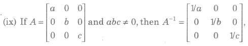
9. Adjoint of a diagonal matrix is a diagonal matrix.

Inverse of a Square Matrix

Let A be a square matrix of order n, then a square matrix B, such that AB = BA = I, is called inverse of A, denoted by A^-1.

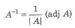
i.e.,
or AA^-1 = A^-1A = 1

Properties of Inverse of a Square Matrix

1. Square matrix A is invertible if and only if |A| ≠ 0
2. (A^-1)^-1 = A
3. (A’)^-1 = (A^-1)’
4. (AB)^-1 = B^-1A^-1 In general (A₁A₁A₁ … A_n)^-1 = A_n ^-1A_n – 1 ^-1 … A₃^-1A2 ^-1A₁ ^-1
5. If a non-singular square matrix A is symmetric, then A^-1 is also symmetric.
6. |A^-1| = |A|^-1
7. AA^-1 = A^-1A = I
8. (A^k)^-1 = (A^-1)A^k k ∈ N

Elementary Transformation

Any one of the following operations on a matrix is called an elementary transformation.

1. Interchanging any two rows (or columns), denoted by R_i←→Rj or C_i←→C_j
2. Multiplication of the element of any row (or column) by a non-zero quantity and denoted by R_i → kR_i or C_i → kC_j
3. Addition of constant multiple of the elements of any row to the corresponding elementof any other row, denoted by R_i → R_i + kRj or C_i → C_i + kC_j

Equivalent Matrix

• Two matrices A and B are said to be equivalent, if one can be obtained from the other by a sequence of elementary transformation.
• The symbol≈ is used for equivalence.

Rank of a Matrix

A positive integer r is said to be the rank of a non-zero matrix A, if

1. there exists at least one minor in A of order r which is not zero.
2. every minor in A of order greater than r is zero, rank of a matrix A is denoted by ρ(A) = r.

Properties of Rank of a Matrix

1. The rank of a null matrix is zero ie, ρ(0) = 0
2. If In is an identity matrix of order n, then ρ(I_n) = n.
3. (a) If a matrix A does’t possess any minor of order r, then ρ(A) ≥ r.
(b) If at least one minor of order r of the matrix is not equal to zero, then ρ(A) ≤ r.

4. If every (r + 1)th order minor of A is zero, then any higher order – minor will also be zero.
5. If A is of order n, then for a non-singular matrix A, ρ(A) = n
6. ρ(A’)= ρ(A)
7. ρ(A^*) = ρ(A)
8. ρ(A + B) &LE; ρ(A) + ρ(B)
9. If A and B are two matrices such that the product AB is defined, then rank (AB) cannot exceed the rank of the either matrix.
10. If A and B are square matrix of same order and ρ(A) = ρ(B) = n, then p(AB)= n
11. Every skew-symmetric matrix,of odd order has rank less than its order.
12. Elementary operations do not change the rank of a matrix.

Echelon Form of a Matrix

A non-zero matrix A is said to be in Echelon form, if A satisfies the following conditions

1. All the non-zero rows of A, if any precede the zero rows.
2. The number of zeros preceding the first non-zero element in a row is less than the number of such zeros in the successive row.
3. The first non-zero element in a row is unity.
4. The number of non-zero rows of a matrix given in the Echelon form is its rank.

Homogeneous and Non-Homogeneous System of Linear Equations

A system of equations AX = B, is called a homogeneous system if B = 0 and if B ≠ 0, then it is called a non-homogeneous system of equations.

Solution of System of Linear Equations

The values of the variables satisfying all the linear equations in the system, is called solution of system of linear equations.

1 . Solution of System of Equations by Matrix Method

(i) Non-Homogeneous System of Equations

Let AX = B be a system of n linear equations in n variables.

• If |A| ≠ 0, then the system of equations is consistent and has a unique solution given by X = A^-1B.
• If |A| = 0 and (adj A)B = 0, then the system of equations is consistent and has infinitely many solutions.
• If |A| = 0 and (adj A) B ≠ 0, then the system of equations is inconsistent i.e., having no solution

(ii) Homogeneous System of Equations

Let AX = 0 is a system of n linear equations in n variables.

• If I |A| ≠ 0, then it has only solution X = 0, is called the trivial solution.
• If I |A| = 0, then the system has infinitely many solutions, called non-trivial solution.

2. Solution of System of Equations by Rank Method

(i) Non-Homogeneous System of Equations

Let AX = B, be a system of n linear equations in n variables, then

• Step I Write the augmented matrix [A:B]
• Step II Reduce the augmented matrix to Echelon form using elementary owtransformation.
• Step III Determine the rank of coefficient matrix A and augmented matrix [A:B] by counting the number of non-zero rows in A and [A:B].

 

Important Results

1. If ρ(A) ≠ ρ(AB), then the system of equations is inconsistent.
2. If ρ(A) =ρ(AB) = the number of unknowns, then the system of equations is consistent and has a unique solution.
3. If ρ(A) = ρ(AB) < the number of unknowns, then the system of equations is consistent and has infinitely many solutions.

(ii) Homogeneous System of Equations

• If AX = 0, be a homogeneous system of linear equations then, If ρ(A) = number of unknown, then AX = 0, have a non-trivial solution, i.e., X = 0.
• If ρ(A) < number of unknowns, then AX = 0, have a non-trivial solution, with infinitely many solutions.