Let A and B be two non-empty sets, then a function f from set A to set B is a rule which associates each element of A to a unique element of B.

It is represented as f: A → B and function are also called mapping.
f : A → B is called a real function, if A and B are subsets of R.

Domain and Codomain of a Real Function

Domain and codomain of a function f is a set of all real numbers x for which f(x) is a real number. Here, set A is domain and set B is codomain.

Range of a Real Function

Range of a real function, f is a set of values f(x) which it attains on the points of its domain.

Classification of Real Functions

Real functions are generally classified under two categories algebraic functions and transcendental functions.

1. Algebraic Functions

Some algebraic functions are given below
(i) Polynomial Functions If a function y = f(x) is given by

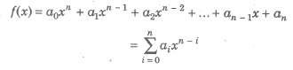
where, a₀, a₁, a₂,…, a_n are real numbers and n is any non -negative integer, then f (x) is called a polynomial function in x.

If a₀ ≠ 0, then the degree of the polynomial f(x) is n. The domain of a polynomial function is the set of real number R.

e.g., y = f(x) = 3x⁵ – 4x² – 2x +1

is a polynomial of degree 5.

 

(ii) Rational Functions If a function y = f(x) is given by f(x) = φ(x) / Ψ(x)

where, φ(x) and Ψ(x) are polynomial functions, then f(x) is called rational function in x.

(iii) Irrational Functions The algebraic functions containing one or more terms having nonintegral rational power x are called irrational functions.
e.g., y = f(x) = 2√x –³√x + 6

2. Transcendental Function

A. function, which is not algebraic, is called a transcendental function. Trigonometric, Inverse trigonometric, Exponential, Logarithmic, etc are transcendental functions.

Explicit and Implicit Functions

(i) Explicit Functions A function is said to be an explicit function, if it is expressed in the form y = f(x).

(ii) Implicit Functions A function is said to be an implicit function, if it is expressed in the form f(x, y) = C, where C is constant.
e.g., sin (x + y) – cos (x + y) = 2

Intervals of a Function

(i) The set of real numbers x, such that a ≤ x ≤ b is called a closed interval and denoted by [a, b] i.e., {x: x ∈ R, a ≤ x ≤ b}.

(ii) Set of real number x, such that a < x < b is called open interval and is denoted by (a, b) i.e., {x: x ∈ R, a < x < b}

(iii) Intervals [a,b) = {x: x ∈ R, a ≤ x ≤ b} and (a, b] = {x: x ≠ R, a < x ≤ b} are called semiopen and semi-closed intervals.

Graph of Real Functions

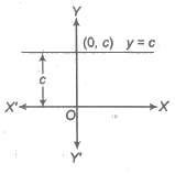
1. Constant Function Let c be a fixed real number.

The function that associates to each real number x, this fixed number c is called a constant function i.e., y = f{x) = c for all x ∈ R.

Domain of f{x) = R
Range of f{x) = {c}

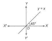
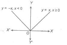
2. Identity Function

The function that associates to each real number x for the same number x, is called the identity function. i.e., y = f(x) = x, ∀ x ∈

R. Domain of f(x) = R
Range f(x) = R

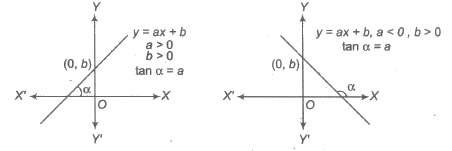
3. Linear Function

If a and b be fixed real numbers, then the linear function is defmed as y = f(x) = ax + b, where a and b are constants.

Domain of f(x) = R
Range of f(x) = R

The graph of a linear function is given in the following diagram, which is a straight line with slope a.

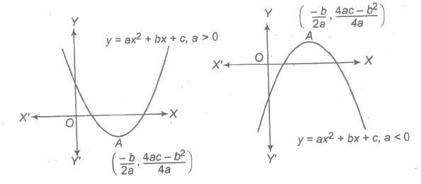
4. Quadratic Function

If a, b and c are fixed real numbers, then the quadratic function is expressed as y = f(x) = ax² + bx + c, a ≠ 0 ⇒ y = a (x + b / 2a)² + 4ac – b² / 4a

which is equation of a parabola in downward, if a < 0 and upward, if a > 0 and vertex at ( – b / 2a, 4ac – b² / 4a).

Domain of f(x) = R

Range of f(x) is [ – ∞, 4ac – b² / 4a], if a < 0 and [4ac – b² / 4a, ∞], if a > 0 5. Square Root Function Square root function is defined by y = F(x) = √x, x ≥ 0.

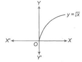
5. Square Root Function

Square root function is defined by y = F(x) = √x, x ≥ 0.

Domain of f(x) = [0, ∞)
Range of f(x) = [0, ∞)

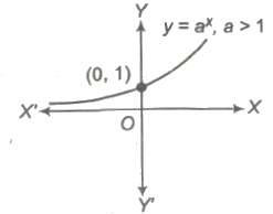
6. Exponential Function

Exponential function is given by y = f(x) = a^x, where a > 0, a ≠ 1.

7. Logarithmic Function

A logarithmic function may be given by y = f(x) = loga x, where a > 0, a ≠ 1 and x > 0.

The graph of the function is as shown below. which is increasing, if a > 1 and decreasing, if 0 < a < 1.

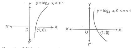
Domain of f(x) = (0, ∞)
Range of f(x) = R

8. Power Function

The power function is given by y = f(x) = xⁿ ,n ∈ I,n≠ 1, 0. The domain and range of the graph y = f(x), is depend on n.

(a) If n is positive even integer.

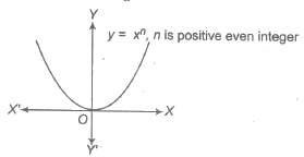
i.e., f(x) = x², x⁴ ,….

Domain of f(x) = R
Range of f(x) = [0, ∞)

(b) If n is positive odd integer.

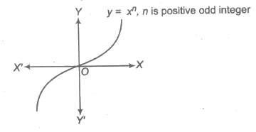
i.e., f(x) = x³, x⁵ ,….

Domain of f(x) = R
Range of f(x) = R

(c) If n is negative even integer.

i.e., f(x) = x^{– 2}, x ^{– 4} ,….

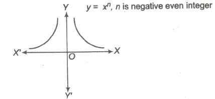
Domain of f(x) = R – {0}
Range of f(x) = (0, ∞)

(d) If n is negative odd integer.

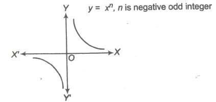
i.e., f(x) = x^{– 1}, x ^{– 3} ,….

Domain of f(x) = R – {0}
Range of f(x) = R – {0}

 

9. Modulus Function (Absolute Value Function)

Modulus function is given by y = f(x) = |x| , where |x| denotes the absolute value of x, that is

|x| = {x, if x ≥ 0, – x, if x < 0

Domain of f(x) = R
Range of f(x) = [0, &infi;)

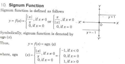
Domain of f(x) = R
Range of f(x) = {-1, 0, 1}

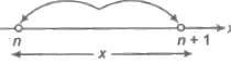
11. Greatest Integer Function

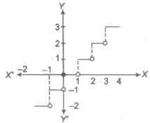
The greatest integer function is defined as y = f(x) = [x]

where, [x] represents the greatest integer less than or equal to x. i.e., for any integer n, [x] = n, if n ≤ x < n + 1 Domain of f(x) = R Range of f(x) = I

Properties of Greatest Integer Function

(i) [x + n] = n + [x], n ∈ I
(ii) x = [x] + {x}, {x} denotes the fractional part of x.
(iii) [- x] = – [x], -x ∈ I
(iv) [- x] = – [x] – 1, x ∈ I
(v) [x] ≥ n ⇒ x ≥ n,n ∈ I
(vi) [x] > n ⇒ x ⇒ n+1, n ∈ I
(vii) [x] ≤ n ⇒ x < n + 1, n ∈ I
(viii) [x] < n ⇒ x < n, n ∈ I
(ix) [x + y] = [x] + [y + x – [x}] for all x, y ∈ R
(x) [x + y] ≥ [x] + [y]
(xi) [x] + [x + 1 / n] + [x + 2 / n] +…+ [x + n – 1 / n] = [nx], n ∈ N

12. Least Integer Function

The least integer function which is greater than or equal to x and it is denoted by (x). Thus, (3.578) = 4, (0.87) = 1, (4) = 4, (- 8.239) = – 8, (- 0.7) = 0

In general, if n is an integer and x is any real number between n and (n + 1).
i.e., n < x ≤ n + 1, then (x) = n + 1

∴ f(x) = (x)

Domain of f = R
Range of f= [x] + 1

13. Fractional Part Function

It is denoted as f(x) = {x} and defined as

(i) {x} = f, if x = n + f, where n ∈ I and 0 ≤ f < 1
(ii) {x} = x – [x]

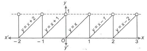
i.e., {O.7} = 0.7, {3} = 0, { – 3.6} = 0.4
(iii) {x} = x, if 0 ≤ x ≤ 1
(iv) {x} = 0, if x ∈ I
(v) { – x} = 1 – {x}, if x ≠ I

Graph of Trigonometric Functions

1. Graph of sin x

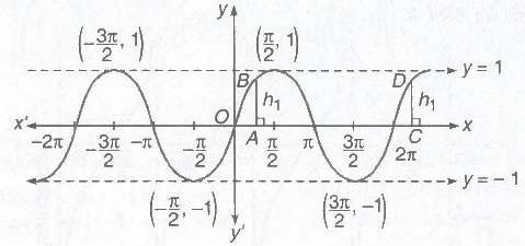
(i) Domain = R
(ii) Range = [-1,1]
(iii) Period = 2π

2. Graph of cos x

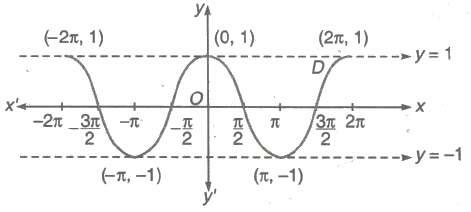
(i) Domain = R
(ii) Range = [-1,1]
(iii) Period = 2π

3.Graph of tan x

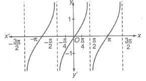
(i) Domain = R ~ (2n + 1) π / 2, n ∈ I
(ii) Range = [- &infi;, &infi;]
(iii) Period = π

4. Graph of cot x

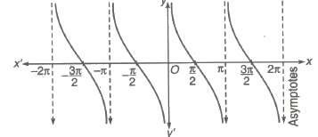
(i) Domain = R ~ nπ, n ∈ I
(ii) Range = [- &infi;, &infi;]
(iii) Period = π

5. Graph of sec x

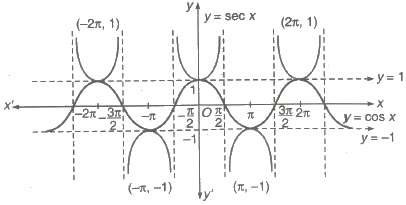
(i) Domain = R ~ (2n + 1) π / 2, n ∈ I
(ii) Range = [- &infi;, 1] ∪ [1, &infi;)
(iii) Period = 2π

6. Graph of cosec x

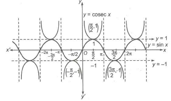
(i) Domain = R ~ nπ, n ∈ I
(ii) Range = [- &infi;, – 1] ∪ [1, &infi;)
(iii) Period = 2π

Operations on Real Functions

Let f: x → R and g : X → R be two real functions, then

(i) Sum The sum of the functions f and g is defined as f + g : X → R such that (f + g) (x) = f(x) + g(x).
(ii) Product The product of the functions f and g is defined as fg : X → R, such that (fg) (x) = f(x) g(x) Clearly, f + g and fg are defined only, if f and g have the same domain. In case, the domain of f and g are different. Then, Domain of f + g or fg = Domain of f ∩ Domain of g.
(iii) Multiplication by a Number Let f : X → R be a function and let e be a real number .
Then, we define cf: X → R, such that (cf) (x) = cf (x), ∀ x ∈ X.
(iv) Composition (Function of Function) Let f : A → B and g : B → C be two functions. We define gof : A → C, such that got (c) = g(f(x)), ∀ x ∈ A
Alternate There exists Y ∈ B, such that if f(x) = y and g(y) = z, then got (x) = z

Periodic Functions

A function f(x) is said to be a periodic function of x, provided there exists a real number T > 0, such that F(T + x) = f(x), ∀ x ∈ R

The smallest positive real number T, satisfying the above condition is known as the period or the fundamental period of f(x) ..

 

Testing the Periodicity of a Function

(i) Put f(T + x) = f(x) and solve this equation to find the positive values of T independent of x.
(ii) If no positive value of T independent of x is obtained, then f(x) is a non-periodic function.
(iii) If positive val~es ofT independent of x are obtained, then f(x) is a periodic function and the least positive value of T is the period of the function f(x).

Important Points to be Remembered

(i) Constant function is periodic with no fundamental period.
(ii) If f(x) is periodic with period T, then 1 / f(x) and. √f(x) are also periodic with f(x) same period T.
{iii} If f(x) is periodic with period T₁ and g(x) is periodic with period T₂, then f(x) + g(x) is periodic with period equal to LCM of T₁ and T₂, provided there is no positive k, such that f(k + x) = g(x) and g(k + x) = f(x).
(iv) If f(x) is periodic with period T, then kf (ax + b) is periodic with period T / |a|’ where a, b ,k ∈ R and a, k ≠ 0.
(v) sin x, cos x, sec x and cosec x are periodic functions with period 2π.
(vi) tan x and cot x are periodic functions with period π.
(vii) |sin x|, |cos x|, |tan x|, |cot x|, |sec x| and |cosec x| are periodic functions with period π.
(viii) sinⁿ x, cosⁿ x, secⁿ x and cosecⁿx are periodic functions with period 2π when n is odd, or π when n is even .
(ix) tanⁿ x and cotⁿx are periodic functions with period π.
(x) |sin x| + |cos x|, |tan x| + |cot x| and |sec x| + |cosec x| are periodic with period π / 2.

Even and Odd Functions

Even Functions A real function f(x) is an even function, if f( -x) = f(x).
Odd Functions A real function f(x) is an odd function, if f( -x) = – f(x).

Properties of Even and Odd Functions

(i) Even function ± Even function = Even function.
(ii) Odd function ± Odd function = Odd function.
(iii) Even function * Odd function = Odd function.
(iv) Even function * Even function = Even function.
(v) Odd function * Odd function = Even function.
(vi) gof or fog is even, if anyone of f and g or both are even.
(vii) gof or fog is odd, if both of f and g are odd.
(viii) If f(x) is an even function, then d / dx f(x) or ∫ f(x) dx is odd and if dx .. f(x) is an odd function, then d / dx f(x) or ∫ f(x) dx is even.
(ix) The graph of an even function is symmetrical about Y-axis.
(x) The graph of an odd function is symmetrical about origin or symmetrical in opposite quadrants.
(xi) An even function can never be one-one, however an odd function mayor may not be oneone.

Different Types of Functions (Mappings)

1. One-One and Many-One Function

The mapping f: A → B is a called one-one function, if different elements in A have different images in B. Such a mapping is known as injective function or an injection.

Methods to Test One-One

(i) Analytically If x₁, x₂ ∈ A, then f(x₁) = f(x₂) => x₁ = x₂ or equivalently x₁ ≠ x₂ => f(x₁) ≠ f(x₂)
(ii) Graphically If any .line parallel to x-axis cuts the graph of the function atmost at one point, then the function is one-one.
(iii) Monotonically Any function, which is entirely increasing or decreasing in whole domain, then f(x) is one-one.
Number of One-One Functions Let f : A → B be a function, such that A and B are finite sets having m and n elements respectively, (where, n > m).
The number of one-one functions n(n – 1)(n – 2) …(n – m + 1) = { ⁿP_m, n ≥ m, 0, n < m
The function f : A → B is called many – one function, if two or more than two different elements in A have the same image in B.

2. Onto (Surjective) and Into Function

If the function f: A → B is such that each element in B (codomain) is the image of atleast one element of A, then we say that f is a function of A ‘onto’ B.
Thus, f: A → B, such that f(A) = i.e., Range = Codomain Note Every polynomial function f: R → R of degree odd is onto.
Number of Onto (surjective) Functions Let A and B are finite sets having m and n elements respectively, such that 1 ≤ n ≤ m, then number of onto (surjective) functions from A to B is ⁿΣ_r = 1 (- 1)^{n – r n}C_r r^m = Coefficient ofⁿ in n! (e^x – 1)^r If f : A → B is such that there exists atleast one element in codomain which is not the image of
Thus, f : A → B, such that f(A) ⊂ B
i.e., Range ⊂ Codomain

 

Important Points to be Remembered

(i) If f and g are injective, then fog and gof are injective.
(ii) If f and g are surjective, then fog is surjective.
(iii) Iff and g are bijective, then fog is bijective.

Inverse of a Function

Let f : A → B is a bijective function, i.e., it is one-one and onto function.

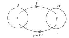
We define g : B → A, such that f(x) = y => g(y) = x, g is called inverse of f and vice-versa.
Symbolically, we write g = f-1
Thus, f(x) = y => f^-1(y) = x